ADIDAS SALES DATA ANALYSIS PROJECT

Project Description:

This is a simple descriptive analysis project based on Adidas sales data provided from Kaggle.com for the years 2020 and 2021.

The goal of this project was to display my reporting capabilities through the development of an excel report that provides an overview of sales performance while also tracking performance over time for each state, store, and product in an attempt to identify insights within the data.

Tools Used In This Project:

Microsoft Excel: used to explore, clean, analyse, and visualize the data.

Problem Statement:

This project was developed with the assumption that the stakeholders require an in-depth sales performance analysis report with sales tracking through 2020 - 2021.

Phase 1: Asking The Right Questions:

I designed the analysis report to provide responses to the following questions:

How did our sales performance compare between 2020 and 2021?
Who is our top retailer overall, and who is our top retailer each year?
What were the largest and lowest sales reported for each year, as well as our top and worst five states and cities?
What is our best-selling product?
Who sells the most of each type of payment?

Dataset:

The dataset was a single .xlsx format file that contained Over 9,000 records of Adidas sales data for the years 2020 and 2021, and it consisted of the 12 columns listed below:

Retailer
Retailer ID
Invoice Date
Region
State
City
Product
Price per Unit
Units Sold
Total Sales
Operating Profit
Sales Method

Phase 2: Data Exploring, Preparing & Cleaning:

I Followed the following steps to look for problems within the data:

Creating a copy of the original raw data.
Removing the rows that contains the title and logo from the set.
Formatting the data as a table by highlighting all the data and pressing the shortcut CTRL+T.
Renaming the table as "Data".
Extracting the year, month, and weekday from the order date:
- This was done using the "YEAR" and "TEXT" functions respectively:

Categorizing Products Into "Men" & "Women" Products:

This was done to add another analysis prospective by looking at sales by gender. This was achieved by using a combination of the "LEFT" and "IF" functions, and the formula was:

=IF(LEFT([@Product],1)="M","Men's Product","Women's Product")

Searching For Blanks within the data:

This was achieved by selecting all of the data and using the "Go To Special" feature of excel:

The results of the previous step showed that there were some null values within the price data. This problem was solved by writing a formula that checks whether the cell contained a null value or not, and calculates the price per unit for the empty cells based on the equation:

Equation: Price per unit = ( Total Sales - Operating Profit ) / Units Sold

The formula used to perform this step was:

Formula: =IF([@[Price per Unit]]="",([@[Total Sales]]-[@[Operating Profit]])/[@[Units Sold]],[@[Price per Unit]])

The preceding step's results additionally pointed to a presence of null values within the region data. While these values might have been entered manually, I took this approach to resolve the problem:

Identifying and recording the regions of the states with missing region data in a table.
utilising the "Create From Selection" feature of Excel to create name ranges for the states and regions data to avoid utilising mixed and absolute references when matching the missing values with the proper values.
To achieve the matching, use a "INDEX-MATCH" technique in conjunction with a "IF" function like follows:
- Formula: =IF([@Region]="",INDEX(State,MATCH([@Region],Region,0)),[@Region])

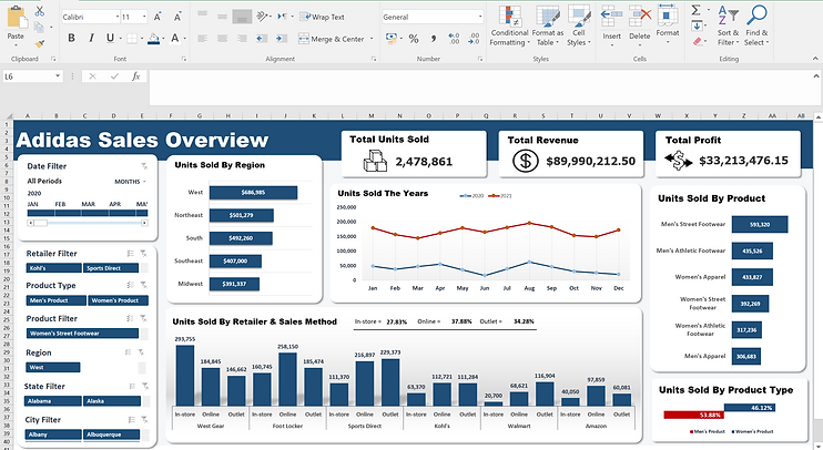
Phase 3: Conducting The Analysis & Creating The Dashboard:

I started to prepare the overview section of the report by building pivot tables in one sheet and "this sheet was hidden" to calculate the followings:

Total Sales.
Total Profit.
Total Units Sold.
Sales by region sorted in a descending order.
Sales by product sorted in a descending order.
Sales by product type.
Sales by retailer and sales method.
Sales by date and using "YEAR" as legend.

These pivot tables were used to construct the dashboard, and slicers were utilised for adding interactivity:

Phase 4: Building The Performance Breakdown By Retailer & Year Section:

The previous image displays the monthly sales performance split for each retailer, product, and year. I took the following procedures to create this section of the report:

Using "data validation" feature to build a dropdown lists of the retailer and year data that enable the report's consumers to select specific retailer or year and read the results.
Calculating the quantity sold (Units sold) for each month using the "SUMIFS" function that incorporates a mixed reference as follows:
- =SUMIFS(Units_Sold,Retailer,$F$6,Year,$I$6,Month,C$14)
Calculating the total revenue (total sales) for each month using the "SUMIFS" function that incorporates a mixed reference as follows:
- =SUMIFS(Total_Sales,Retailer,$F$6,Year,$I$6,Month,C$14)
Calculating the total profit (total operating profit) for each month using the "SUMIFS" function that incorporates a mixed reference as follows:
- =SUMIFS(Operating_Profit,Retailer,$F$6,Year,$I$6,Month,C$14)
Calculating the total number of units sold in the second section of the sheet using a similar technique of the "SUMIFS" function:
- =SUMIFS(Units_Sold,Product,$B21,Retailer,$F$6,Year,$I$6,Month,C$28)
Calculating the total number of units sold of men's and women's product with the formulas:
- =SUMIFS(Units_Sold,Product_Type,"Men's Product",Year,$I$6,Retailer,$F$6)
- =SUMIFS(Units_Sold,Product_Type,"Women's Product",Year,$I$6,Retailer,$F$6)
Using trend lines to demonstrate sales fluctuation over the months.
Calculating the overall total using the formula with the mixed reference:
- =SUM($C10:$N10)
Calculating the overall average using the formula with the mixed reference:
- =$P11/COLUMNS($C11:$N11)
Using the "Conditional Formatting" feature to highlight rises in sales with green colour and drops with red colour using the formula:
- =$D10>$C10
Using the "Conditional Formatting" feature to highlight #1 product by units sold with green colour using the formula:
- =RANK.AVG($P21,$P$21:$P$26,0)=1

Phase 5: Building The Sales By City 5 Cities Section:

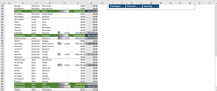
The previous images show the top 5 cities in terms of units sold, with slicers added for better emphasis. I took the following procedures to create this component of the report:

Using "data validation" feature to build a dropdown lists of the retailer and year data that enable the report's consumers to select specific retailer or year and read the results.
Calculating the quantity sold (Units sold) for each city using the "SUMIFS" function that incorporates a mixed reference as follows:
- =SUMIFS(Units_Sold,Retailer,$F$6,Year,$I$6,City,$B35)
Calculating sales amount for each city using the "SUMIFS" function that incorporates a mixed reference as follows:
- =SUMIFS(Total_Sales,Retailer,$F$6,Year,$I$6,City,$B35)
Calculating profit amount (total operating profit) for each city using the "SUMIFS" function that incorporates a mixed reference as follows:
- =SUMIFS(Operating_Profit,Retailer,$F$6,Year,$I$6,City,$B35)
Using the "Conditional Formatting" feature to highlight the tot 5 cities by units sold with green colour and white font using the formula:
- =RANK.AVG($E35,$E$35:$E$86,0)<=5
Using the "Heatmap in Conditional Formatting" feature on the profit column to highlight values based on there amount with a scale that goes from light grey for the low values to dark grey for the high values.
Using the "Conditional Formatting" feature to add data bars to the units sold column for more effective reading.
Formatting the cities data as a table and inserting slicers for both region and state.

Phase 6: Building The Summary Section:

The preceding images provide a summary of sales changes for each state, retailer, and product, with demonstration of the best and worst. For creating this summary report, I used the following procedures:

Calculating the sales for each state, retailer, and product using "SUMIFS" functions with references similar to the previous ones used in the previous section:
- For states: Formula used: =SUMIFS(Units_Sold,State,B11,Year,$C$9)
- For Retailers: Formula used: =SUMIFS(Units_Sold,Retailer,J24,Year,$K$22)
- For Products: Formula used: =SUMIFS(Units_Sold,Product,J11,Year,$K$9)
Calculating the Sales change % for states, retailers, and products with formulas that uses the "IFERROR" function to return "0" in the case of dividing by zero:
- For states: Formula used: =IFERROR((E11/C11)-1,0)
- For Retailers: Formula used: =IFERROR((M24/K24)-1,0)
- For Products: Formula used: =IFERROR((M11/K11)-1,0)
Highlighting the top 5 growing (Higher sale change %) states using the same "Conditional Formatting" technique used to highlight the top 5 cities in the previous stage, with the addition of highlighting the bottom 5 states with red colour using the formula:
- =$G11<0
Highlighting the #1 growing retailer and product using using the same "Conditional Formatting" technique used to highlight the #1 retailer in the previous stage.

Download The Final Report:

You may download and view the final report by clicking on the download button below.

Note: The report has been password-protected to prevent unauthorised alterations. Please contact me if you require removal of the protection and full access to the report.

Download Report

References:

Dataset: Adidas Sales Dataset. (n.d.). Adidas Sales Dataset | Kaggle. https:///datasets/heemalichaudhari/adidas-sales-dataset

Adidas Image: W. (2022, July 27). Slow recovery in China, slowdowns cause Adidas to adjust FY22 outlook. Slow Recovery in China, Slowdowns Cause Adidas to Adjust FY22 Outlook - Fibre2Fashion. http://www.fibre2fashion.com/news/retail-industry/slow-recovery-in-china-slowdowns-cause-adidas-to-adjust-fy22-outlook-282140-newsdetails.htm